Multi-Head Attention: The Engine of Parallel Representation in Transformers

This is the perfect next question. If the scaled dot-product attention is the "engine" that powers the Transformer, Multi-Head Attention is the transmission system that allows it to operate across multiple gears at the same time.

Here is a breakdown of what it is, the math behind it, and the conceptual reasons why it is absolutely critical for modern LLMs.

1. What is Multi-Head Attention?

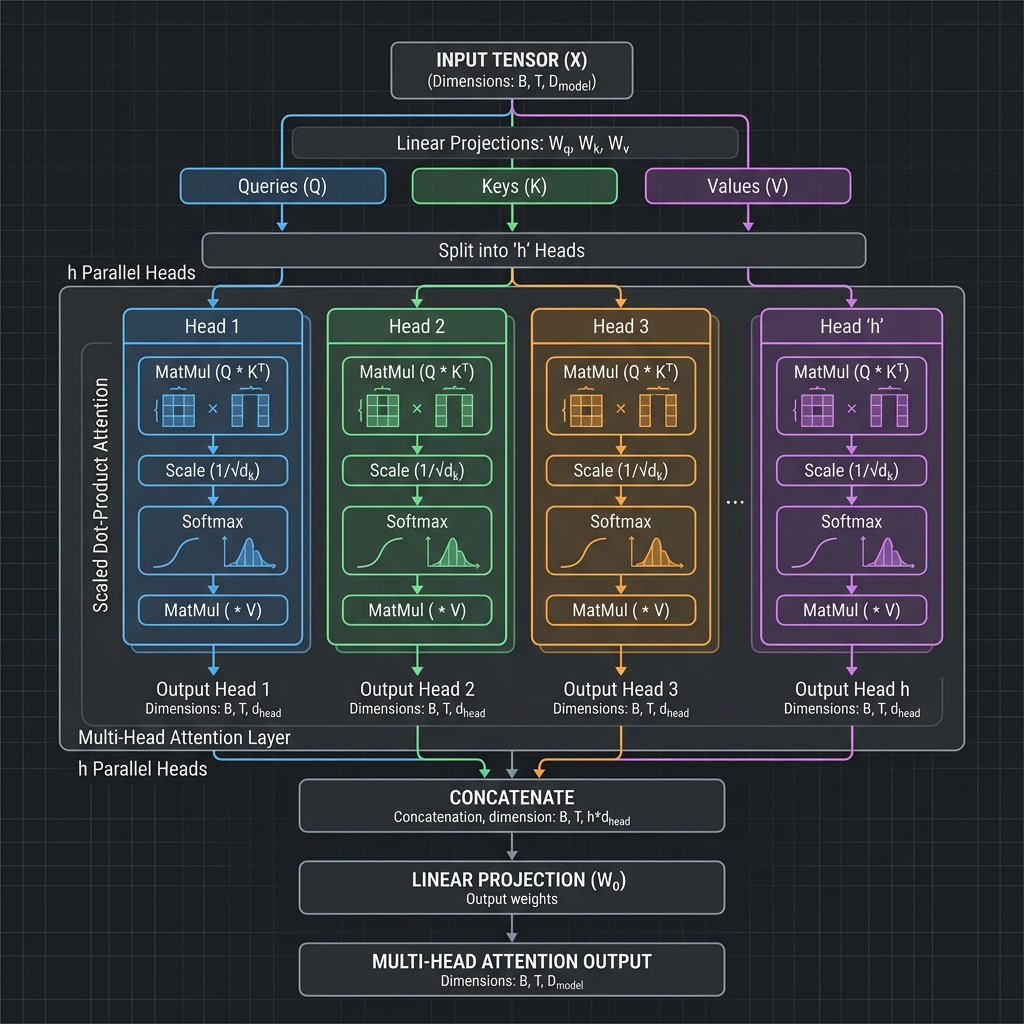
In a single-head attention mechanism, you have one set of Query ($Q$), Key ($K$), and Value ($V$) matrices. The model calculates the attention scores once and produces a single output sequence.

Multi-Head Attention splits this process into multiple parallel tracks (called "heads"). Instead of computing attention once on the full, high-dimensional vectors, the model linearly projects the $Q$, $K$, and $V$ matrices into $h$ different, smaller "subspaces." It then performs the scaled dot-product attention independently on each of these $h$ subspaces.

Mathematically, it looks like this:

For each head $i$ (from 1 to $h$): $\text{head}_i = \text{Attention}(QW_i^Q, KW_i^K, VW_i^V)$

(Where $W_i^Q, W_i^K, W_i^V$ are distinct, learned weight matrices that project the data into smaller dimensions).

Finally, all the outputs from the independent heads are concatenated (glued back together) and multiplied by a final weight matrix ($W^O$) to return to the original dimension: $\text{MultiHead}(Q, K, V) = \text{Concat}(\text{head}_1, \dots, \text{head}_h)W^O$

2. Why use Multiple Heads? (The "Why")

If we have a powerful single attention mechanism, why bother splitting it up? There are two primary reasons:

Reason A: Capturing Different "Representation Subspaces"

Human language is deeply complex. A single word in a sentence has multiple relationships with the words around it simultaneously. Take the sentence: "The animal didn't cross the street because it was too tired." What should the word "it" pay attention to?

• Grammatically: "it" is the subject of the verb "was".
• Semantically (Coreference): "it" refers to the "animal" (not the street).
• Descriptively: "it" is connected to the state of being "tired".

If you only have one attention head, the model has to squish all of these distinct relationships into a single weighted average. The attention signal becomes muddy and compromised.

By having multiple heads, the model delegates tasks. Head 1 can become the "Grammar Head" looking at verbs, Head 2 can become the "Pronoun Resolution Head" linking "it" to "animal", and Head 3 can be the "Adjective Head". They all operate in their own specialized subspaces without interfering with one another.

Reason B: Preventing the "Blurring" Effect

Softmax naturally wants to create a sharp distribution (paying a lot of attention to one or two words and ignoring the rest). If a single attention head is forced to look at the subject, the verb, and the adjective all at once, the Softmax probabilities get averaged out (e.g., 33% to each). This "blurring" destroys the sharpness of the neural network's focus.

Multiple heads allow each individual Softmax calculation to remain incredibly sharp and opinionated about its specific task, while the concatenation at the end ensures the model gets the full, nuanced picture.

---

The "Panel of Experts" Analogy

Imagine you are evaluating a movie.

• If you send one general critic (Single-Head Attention), they will give you a single, averaged review: "The plot was okay, the music was good, the acting was fine. 7/10." You lose the specific details.
• If you send a panel of experts (Multi-Head Attention)—a cinematographer, a composer, a scriptwriter, and a costume designer—they each watch the exact same movie (the input data), but they project their attention onto completely different aspects. When you combine their reports (Concatenation), you get an incredibly rich, multi-dimensional understanding of the film.

To make this completely intuitive, let's walk through a simplistic Toy Example.

We will compute Multi-Head Attention for a short sequence composed of two words: "Cat sleeps".

📝 Problem Setup

• Sequence length: 2 ("Cat" and "sleeps").
• Embedding Dimension ($d_{model}$): 4 dimensions (Each word is encoded as a 4-number vector).
• Number of Heads ($h$): 2 Heads (We have 2 "experts").
• Head Dimension ($d_k = d_v$): $4 / 2 = 2$ dimensions.

---

Step 1: Input Matrix ($X$)

Assume that after the Embedding layer, our two words form the matrix $X$ (dimensions $2 \times 4$): $X = \begin{bmatrix} 1 & 2 & 0 & 0 \\ 0 & 0 & 1 & 2 \end{bmatrix} \begin{matrix} \leftarrow \text{"Cat"} \\ \leftarrow \text{"sleeps"} \end{matrix}$ Note: You can easily observe that "Cat" carries information in the first two columns, while "sleeps" carries information in the last two columns.

---

Step 2: Generating Q, K, V per Head (Linear Projection)

The model does not use the full 4-dimensional $X$ directly. It uses weight matrices $W^Q, W^K, W^V$ to project $X$ down to 2 dimensions for each Head.

🎯 Head 1 (Grammar Expert - Focuses on the first two columns): Assume Head 1's weight matrices are trained to extract only the first two columns. When $X$ is multiplied by the matrices $W_1$, we obtain $Q_1, K_1, V_1$ for Head 1 (dimensions $2 \times 2$): $Q_1 = K_1 = V_1 = \begin{bmatrix} 1 & 2 \\ 0 & 0 \end{bmatrix} \begin{matrix} \leftarrow \text{"Cat"} \\ \leftarrow \text{"sleeps"} \end{matrix}$

🎯 Head 2 (Semantics Expert - Focuses on the last two columns): Similarly, Head 2's weight matrices extract the last two columns of $X$: $Q_2 = K_2 = V_2 = \begin{bmatrix} 0 & 0 \\ 1 & 2 \end{bmatrix} \begin{matrix} \leftarrow \text{"Cat"} \\ \leftarrow \text{"sleeps"} \end{matrix}$

---

Step 3: Independent Attention Computation

Now, both Heads operate in parallel, entirely independently. We apply the standard formula: $\text{softmax}\left(\frac{QK^T}{\sqrt{d_k}}\right)V$

Calculation for Head 1:

1. Multiply $Q_1 \cdot K_1^T$ (Similarity Scoring): $\begin{bmatrix} 1 & 2 \\ 0 & 0 \end{bmatrix} \times \begin{bmatrix} 1 & 0 \\ 2 & 0 \end{bmatrix} = \begin{bmatrix} 5 & 0 \\ 0 & 0 \end{bmatrix}$ (The word "Cat" pays high attention to itself with a score of 5, and pays 0 attention to "sleeps").

2. Scale by $\sqrt{d_k}$: Since $d_k = 2 \rightarrow \sqrt{2} \approx 1.41$. $\begin{bmatrix} 5/1.41 & 0 \\ 0 & 0 \end{bmatrix} \approx \begin{bmatrix} 3.5 & 0 \\ 0 & 0 \end{bmatrix}$

3. Softmax (Conversion to Probabilities):

   • Row 1 (Cat): $e^{3.5}$ strictly dominates $e^0$, resulting in approximately [0.97, 0.03] (97% attention to Cat, 3% to sleeps).
   • Row 2 (sleeps): $e^0$ and $e^0$ are equal, resulting in [0.5, 0.5] (50/50). $\text{Softmax}_1 = \begin{bmatrix} 0.97 & 0.03 \\ 0.5 & 0.5 \end{bmatrix}$

4. Multiply by $V_1$ (Information Extraction): $\text{Head}_1 = \begin{bmatrix} 0.97 & 0.03 \\ 0.5 & 0.5 \end{bmatrix} \times \begin{bmatrix} 1 & 2 \\ 0 & 0 \end{bmatrix} = \begin{bmatrix} 0.97 & 1.94 \\ 0.50 & 1.00 \end{bmatrix}$

Calculation for Head 2: Following the exact same procedure but with Head 2's matrices. Because the non-zero data resides entirely in the bottom row, the result will be inverted: $\text{Head}_2 = \begin{bmatrix} 0.00 & 0.00 \\ 0.97 & 1.94 \end{bmatrix}$ (In this subspace, "Cat" extracts no meaningful information, while "sleeps" extracts a very strong signal).

---

Step 4: Component Concatenation

We now stitch the findings from "Expert 1" and "Expert 2" back together horizontally.

• $Head_1$ dimensions are $2 \times 2$.
• $Head_2$ dimensions are $2 \times 2$. Concatenating them produces matrix $Z$ with dimensions $2 \times 4$ (matching the original dimensions of input $X$).

$Z = \text{Concat}(\text{Head}_1, \text{Head}_2) = \begin{bmatrix} 0.97 & 1.94 & \mathbf{0.00} & \mathbf{0.00} \\ 0.50 & 1.00 & \mathbf{0.97} & \mathbf{1.94} \end{bmatrix}$

---

Step 5: Final Linear Projection ($W^O$)

The matrix $Z$ above currently represents "segregated information" (the left half belongs to Head 1, the right half to Head 2). In the final step, we multiply matrix $Z$ by an output weight matrix $W^O$ (dimensions $4 \times 4$). This matrix serves to "mix" and synthesize the information from all independent Heads into a unified, coherent representation.

$\text{Final Output} = Z \times W^O$

💡 The Mathematical Takeaway

From this numerical walkthrough, we can observe:

• Head 1 exclusively processed the first two columns (representing "Cat").
• Head 2 exclusively processed the last two columns (representing "sleeps").
• If we lacked Multi-Head Attention and used a single Head, the algorithm would have aggressively averaged and merged the features of both "Cat" and "sleeps" prematurely, obfuscating their distinct characteristics.

By dividing the representation space ($d_{model} \rightarrow d_k$) and performing parallel computations, the model does not incur significantly higher hardware costs (since the matrices per Head are proportionally smaller), yet it achieves profoundly greater representational power across multiple semantic dimensions!