Foundations of Recurrent Architectures: Parameter Sharing and Temporal Dynamics

The fundamental abstraction in Recurrent Neural Networks (RNNs) is the mapping of sequential dependencies through Parameter Sharing over Time. Unlike standard Feedforward or Convolutional architectures that operate on fixed-dimensional spatial grids, the RNN architecture is designed to map input sequences of arbitrary length into a continuous latent state space.

This research article formalizes the mathematical transformations within an RNN cell and analyzes the inherent computational constraints of recurrent backpropagation.

---

1. Architectural Formalism and Notation

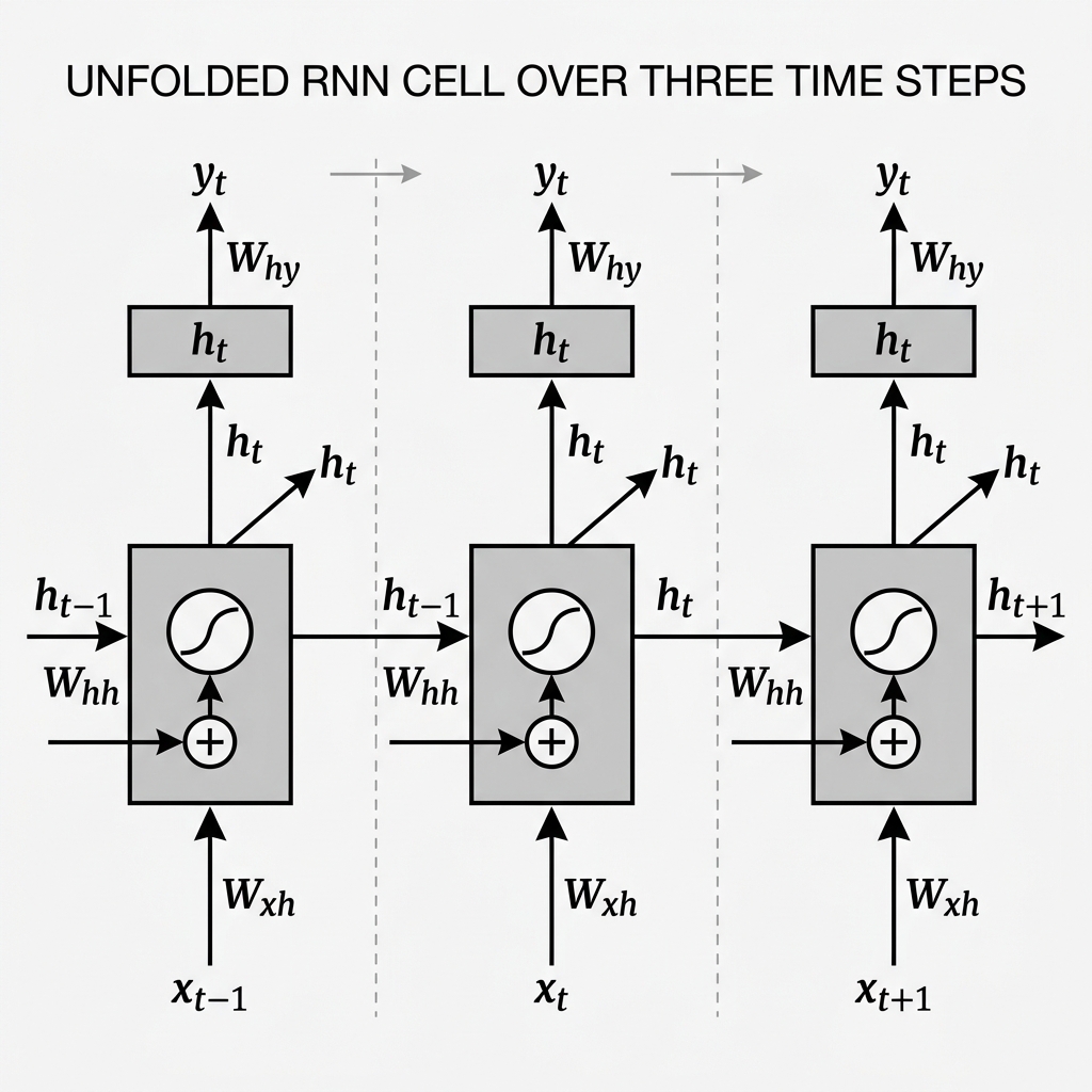
Consider a discrete-time sequence $x = \{x_1, x_2, \dots, x_T\}$, where each $x_t \in \mathbb{R}^d$. The RNN processes this sequence by maintaining an internal Hidden State $h_t \in \mathbb{R}^h$, which acts as a summary of the temporal history up to step $t$.

The system is parameterized by the following weight matrices:

• $W_{xh} \in \mathbb{R}^{h \times d}$: Input-to-Hidden projection.
• $W_{hh} \in \mathbb{R}^{h \times h}$: Recurrent Hidden-to-Hidden transition.
• $W_{hy} \in \mathbb{R}^{k \times h}$: Hidden-to-Output projection.
• $b_h, b_y$: Bias vectors for the hidden and output layers, respectively.

---

2. Temporal State Transitions

At each temporal step $t$, the network executes a dual-stage transformation to update its internal representation and generate an external prediction.

2.1 Hidden State Update (The Recurrent Step)

The transition is governed by a non-linear activation function, typically the hyperbolic tangent ($\tanh$), which squashes the weighted sum of current inputs and previous states:

$h_t = \tanh(W_{xh} x_t + W_{hh} h_{t-1} + b_h)$

Deterministic Memory: The new state $h_t$ is a synthesis of the instantaneous signal $x_t$ and the aggregated historical context $h_{t-1}$. The use of $\tanh$ is mathematically critical to ensure the stability of the latent state, preventing exponential divergence of values during forward propagation.

2.2 Output Projection

The mapping to the label space is performed by projecting the hidden state through the output matrix, often followed by a normalizing transformation such as Softmax for classification:

$y_t = \sigma(W_{hy} h_t + b_y)$

---

3. Mathematical Analysis of Parameter Sharing

A defining characteristic of the RNN is the Temporal Invariance of its parameters. The matrices $\{W_{xh}, W_{hh}, W_{hy}\}$ remain constant across all time-steps $t \in [1, T]$.

This provides two significant advantages:

1. Computational Efficiency: The number of trainable parameters is independent of the input sequence length, allowing the model to generalize across variable temporal scales.
2. Generalization: The model learns a universal "transition rule" that applies regardless of the specific index in the sequence, much like how a Convolutional kernel learns spatial patterns regardless of pixel coordinates.

---

4. The Vanishing Gradient Constraint

The training of RNNs is performed via Backpropagation Through Time (BPTT). When computing the gradient of the loss with respect to the recurrent weights $W_{hh}$, the chain rule spans the entire temporal history:

$\frac{\partial L}{\partial W_{hh}} = \sum_{t=1}^T \frac{\partial L_t}{\partial W_{hh}}$

Evaluating a single term in this summation involves a product of Jacobian matrices: $\frac{\partial h_t}{\partial h_k} = \prod_{i=k+1}^t \frac{\partial h_i}{\partial h_{i-1}} = \prod_{i=k+1}^t W_{hh}^T \text{diag}(\tanh'(W_{xh} x_i + W_{hh} h_{i-1} + b_h))$

Scientific Bottleneck: Since the derivative of the $\tanh$ function is bounded by $[0, 1]$, and the spectral radius of $W_{hh}$ may be small, long temporal chains cause the gradient to decay exponentially toward zero. This results in the Vanishing Gradient Problem, where the network fails to learn long-range dependencies effectively.

---

5. Summary of Recurrent Dynamics

Feature	Deterministic RNN	Analysis
State Mapping	$h_{t-1} \to h_t$	Markovian dependency on immediate past
Activation	$\tanh$	Non-linear stability control
Weight Sharing	Global	Temporal invariance
Optimization	BPTT	Vulnerable to vanishing gradients
Generalization	Variable-length	Agnostic to sequence length

[!CAUTION] Key Limitation: While standard RNNs are mathematically elegant, they are practically unsuitable for sequences exceeding 20-50 steps due to the gradient vanishing bottleneck. This necessitated the development of Gated architectures like LSTMs and GRUs.