Mathematical Foundations of Spatial and Temporal Subsampling: A Study on Pooling Layers

In the design of Deep Convolutional Neural Networks (CNNs), the ability to extract invariant features while controlling computational complexity is paramount. Pooling Layers serve as the mathematical mechanism for spatial and temporal subsampling. Their primary functions include dimensionality reduction, noise attenuation, and the promotion of translation invariance.

This study formalizes the mapping of input tensors to reduced feature spaces across 1D, 2D, and 3D dimensionalities.

---

1. Dimensionality Mapping and Algebraic Formalization

Regardless of the input dimensionality, the transformation of a tensor signal through a pooling operation is governed by the window size $k$, stride $S$, and padding $P$.

General Mapping Function

For an input dimension $D_{in}$, the output dimension $D_{out}$ is calculated as: $D_{out} = \left\lfloor \frac{D_{in} + 2P - k}{S} \right\rfloor + 1$

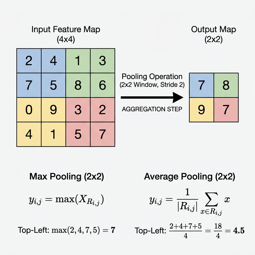
The value of an output element $y_i$ is determined by applying an aggregation function $\mathcal{F}$ over a local subset of the input tensor $\Omega_i$: $y_i = \mathcal{F}(\{x_j \mid j \in \Omega_i\})$

Where $\mathcal{F}$ is defined as:

• Max Pooling: $\mathcal{F}(X) = \max(X)$
• Average Pooling: $\mathcal{F}(X) = \frac{1}{|X|} \sum_{x \in X} x$

---

2. Temporal Subsampling in 1D Architectures

1D Pooling is primarily utilized in sequential signal analysis (e.g., NLP, Telemetry, Audio).

1D Case Study

Consider an input sequence $Input = [1, 5, 2, 8, 3, 6]$ with a pooling window $k=2$ and stride $S=2$.

• MaxPooling1D: Captures local maxima, preserving strong signals or "activations."
  • Output: $[5, 8, 6]$
• AveragePooling1D: Computes the local arithmetic mean, acting as a low-pass filter.
  • Output: $[3, 5, 4.5]$
• GlobalMaxPooling1D: Collapses the entire sequence into a single scalar representing the global maximum activation.
  • Output: $[8]$

---

3. Spatial Subsampling in 2D Architectures

2D Pooling is the standard for image processing and spatial feature map reduction.

2D Formalization

Given an input matrix $M \in \mathbb{R}^{H \times W}$, the output $Y$ is a spatially reduced projection.

$$M = \begin{bmatrix} 1 & 3 & 2 & 1 \\ 5 & \mathbf{9} & 0 & 2 \\ 1 & 0 & \mathbf{8} & 4 \\ 2 & 1 & 3 & 7 \end{bmatrix} \xrightarrow{k=2, S=2, \text{Max}} \begin{bmatrix} 9 & 2 \\ 2 & 8 \end{bmatrix}$$

Scientific Utility: Max pooling is particularly effective for preserving sharp discontinuities such as edges and texture gradients, which are critical for object recognition tasks.

---

4. Volumetric and Spatiotemporal Reduction (3D)

3D Pooling extends the aggregation cube into the volumetric domain, essential for medical imaging (voxels) and video analysis (spatiotemporal blocks).

• Medical Scanning: Reduction of MRI/CT volumes while preserving structural anomalies.
• Action Recognition: Temporal pooling across frames to capture motion invariants while reducing frame-rate dependency.

---

5. Comparative Performance Metrics

Metric	Max Pooling	Average Pooling	Global Pooling
Feature Extraction	Sharp / Extreme signals	Smooth / General trends	Global invariants
Noise Sensitivity	Sensitive to outliers	Robust / Gaussian smoothing	Highly robust
Invariance	Local translation	Local smoothing	Total spatial invariance
Output Shape	Reduced Grid	Reduced Grid	Vector $(1 \times 1 \times C)$

[!TIP] Key Takeaway: Max Pooling is the default for feature extraction in hidden layers, whereas Average/Global Pooling is frequently utilized at the "neck" of the architecture to transition into fully connected classification heads, effectively acting as regularizers against overfitting.