Inverse Diffusion and Latent Manifolds: Formalizing Generative Mechanics in AI Synthesis

In the current paradigm of Artificial Intelligence, Generative AI represents a shift from discriminative classification to a constructive synthesis of high-dimensional data. Rather than simple pattern recognition or heuristic templates, modern generative systems operate by mapping high-entropy noise distributions to low-entropy manifolds of structured information.

This paper formalizes the primary mechanisms of data synthesis, specifically the Diffusion process and Latent Space operations, providing a rigorous mathematical framework for understanding how machines "create" from nothingness.

---

1. Stochastic Prediction: The Foundation of Generative Systems

At their core, all generative models are probabilistic estimation engines. Whether generating text (Large Language Models) or visual information (Diffusion models), the objective is to model the underlying probability distribution $p(x)$ of the training data.

1. Textual Synthesis (Transformers): These models function as autoregressive probability calculators. Given a sequence of tokens $x_{<t}$, the model predicts the conditional probability $p(x_t \mid x_{<t})$. The process is discrete and iterative, where each token is sampled based on a non-linear projection of the preceding context window.
2. Visual Synthesis (Diffusion/GANs): Unlike the discrete steps of text, visual synthesis involves the manipulation of continuous pixel manifolds. The objective is to transform a standard Gaussian noise vector $z \sim \mathcal{N}(0, I)$ into a structured image $x_0$ that satisfies the learned distribution of the visual world.

---

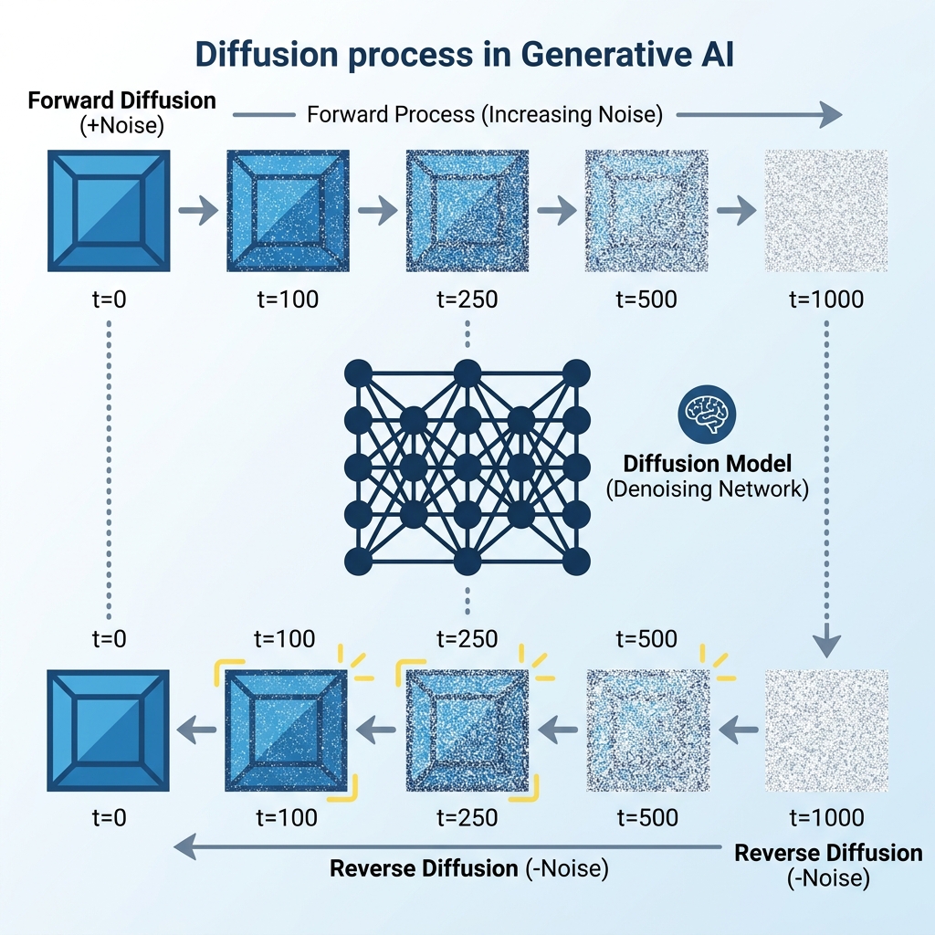
2. Diffusion Dynamics: Sculpting via Denoising

The Diffusion Model (e.g., Stable Diffusion, DALL-E) has become the state-of-the-art mechanism for image generation. Its core logic is counter-intuitive: to teach a model to build an image, one must first teach it how to systematically destroy it.

Forward Diffusion (The Markovian Decay)

During the training phase, an image $x_0$ is progressively corrupted by adding infinitesimal amounts of Gaussian noise $\epsilon$ over $T$ steps (typically $T=1000$). The transition is defined as:

$q(x_t \mid x_{t-1}) = \mathcal{N}(x_t; \sqrt{1-\beta_t} x_{t-1}, \beta_t I)$

As $t \to T$, the original structure vanishes, and the image converges to pure isotropic noise.

Reverse Diffusion (The Generative Inverse)

Synthesis occurs in the reverse direction. Starting from a random noise tensor $x_T$, a neural network $\epsilon_\theta$ predicts the noise component present at each step and subtracts it. The goal is to estimate the reverse transition:

$p_\theta(x_{t-1} \mid x_t) = \mathcal{N}(x_{t-1}; \mu_\theta(x_t, t), \Sigma_\theta(x_t, t))$

The model does not "remember" the image; it learns the score function—the gradient of the log-density that "pushes" the noise toward the high-density regions of the data manifold.

---

3. Numerical Derivation: A $2 \times 2$ Discrete Signal Case Study

To concretize the mechanism, we analyze a simplified case of a $2 \times 2$ grayscale image represented as a matrix $M \in \mathbb{R}^{2 \times 2}$.

Input Configuration

• Target Matrix ($x_0$): A high-contrast "checkered" pattern. $x_0 = \begin{bmatrix} 200 & 50 \\ 50 & 200 \end{bmatrix}$
• Initial Noise ($x_T^{rev}$): A random starting state for synthesis. $x_T^{rev} = \begin{bmatrix} 130 & 80 \\ 90 & 110 \end{bmatrix}$

The Denoising Step

Given the target context (e.g., prompt $y$= "high-contrast pattern"), the model predicts the noise $\hat{\epsilon}$ to be removed.

Iteration 1: The model calculates a gradient to "nudge" the pixels toward the learned pattern: $\hat{\epsilon}_1 = \begin{bmatrix} -30 & 15 \\ 20 & -40 \end{bmatrix}$

Updating the state: $x_{T-1} = x_T - \eta \hat{\epsilon}_1$ (where $\eta$ is a scaling factor). For simplicity: $x_{T-1} = \begin{bmatrix} 130 & 80 \\ 90 & 110 \end{bmatrix} - \begin{bmatrix} -30 & 15 \\ 20 & -40 \end{bmatrix} = \begin{bmatrix} 160 & 65 \\ 70 & 150 \end{bmatrix}$

Iteration 2: The updated state continues to move toward the manifold: $\hat{\epsilon}_2 = \begin{bmatrix} -20 & 10 \\ 15 & -30 \end{bmatrix}$ $x_{T-2} = \begin{bmatrix} 160 & 65 \\ 70 & 150 \end{bmatrix} - \begin{bmatrix} -20 & 10 \\ 15 & -30 \end{bmatrix} = \begin{bmatrix} 180 & 55 \\ 55 & 180 \end{bmatrix}$

By the terminal step, the random noise has been "sculpted" into a matrix that is mathematically indistinguishable from the target $x_0$.

---

4. Adversarial Dynamics: Generative Adversarial Networks (GANs)

Prior to the dominance of Diffusion, GANs utilized a competitive game-theoretic framework. A GAN consists of two networks in a zero-sum game:

1. Generator ($G$): Maps a latent vector $z$ to the data space, $G(z) \to x_{fake}$.
2. Discriminator ($D$): Maps a sample to a probability $D(x) \in [0, 1]$, outputting 1 for real and 0 for fake.

The objective function is defined as: $\min_G \max_D V(D, G) = \mathbb{E}_{x \sim p_{data}(x)}[\log D(x)] + \mathbb{E}_{z \sim p_{z}(z)}[\log(1 - D(G(z)))]$

The system reaches Nash Equilibrium when the Generator produces samples so realistic that $D(x) = 0.5$ for all $x$, indicating total ambiguity.

---

5. Semantic Compression: Latent Manifold Learning

A critical innovation in modern generative systems is the move from Pixel Space to Latent Space. Operating directly on high-resolution pixels ($1024 \times 1024$) is computationally prohibitive.

Generative models utilize a Variational Autoencoder (VAE) to compress the image into a low-dimensional latent representation $z$.

• Chairs, faces, and landscapes become coordinates in this multi-dimensional vector space.
• Arithmetic operations on these vectors correspond to semantic changes (e.g., $Vector(\text{Man}) - Vector(\text{Crown}) = Vector(\text{Woman})$).

By performing the Diffusion process in this compressed latent space (Latent Diffusion), models achieve high-order creativity with manageable compute requirements.

---

6. Architectural Conclusion

Generative AI is not an act of "copying" but of manifold navigation. By leveraging the stochastic calculus of Diffusion and the competitive dynamics of GANs, these architectures learn to traverse the latent manifolds of human knowledge. The transition from noise to signal is a controlled descent into structured probability, enabling machines to synthesize information that is both novel and statistically consistent with our reality.

[!NOTE] Research Insight: The effectiveness of these models relies on the Central Limit Theorem—as noise is added, any distribution eventually becomes Gaussian. By learning to reverse this universal decay, AI captures the fundamental signatures of data structure across all modalities.